Microstrip vs Stripline: Choosing a PCB Routing Structure

Q: Why is a 50 Ω stripline trace narrower than a 50 Ω microstrip trace at the same dielectric distance?

Characteristic impedance is inversely proportional to capacitance per unit length ($Z_0 = \sqrt{L/C}$). Because a stripline conductor is coupled to two reference planes (above and below) inside a higher-permittivity dielectric rather than one plane with air above, it has significantly higher capacitance for a given width. To bring capacitance back down and restore $Z_0 = 50\ \Omega$, the stripline conductor must be made narrower (or the dielectric spacing between planes must be increased).

Q: Why does microstrip have higher far-end crosstalk (FEXT) than symmetric stripline?

In a homogeneous stripline medium, the electric (capacitive) and magnetic (inductive) coupling ratios between two adjacent traces are equal, so odd-mode and even-mode signals travel at the exact same phase velocity ($v_{\text{odd}} = v_{\text{even}}$) and far-end crosstalk cancels out theoretically. In surface microstrip, electric field lines fringe into the air above the board; odd-mode fields have a higher fraction of energy in air than even-mode fields, causing velocity mismatch ($v_{\text{odd}} > v_{\text{even}}$) that produces a large FEXT pulse at the receiver.

Q: How much does solder mask change the impedance of an outer-layer microstrip trace?

Applying standard liquid photoimageable (LPI) solder mask ($15\text{--}30\ \mu\text{m}$ thick, $\varepsilon_r \approx 3.3\text{--}3.8$) over an outer-layer microstrip trace replaces the air interface directly above the conductor with a higher-permittivity dielectric. This typically lowers single-ended characteristic impedance by $2\text{ to }3\ \Omega$ (and differential impedance by $3\text{ to }5\ \Omega$), which must be included in the 2D field-solver model before sizing the trace width.

Compare microstrip and stripline PCB transmission lines across impedance geometry, effective permittivity, propagation delay, far-end crosstalk (FEXT), via stubs, and layer stackup cost.

TechnologyOctober 30, 202612 min read

Microstrip vs Stripline: Choosing a PCB Routing Structure

Choosing between microstrip and stripline routing is not a matter of picking a fixed frequency threshold where one topology automatically replaces the other; it is a stackup and channel-architecture tradeoff between outer-layer component access with zero via transitions (microstrip) and homogeneous dielectric shielding with dual reference planes (stripline).

Because a surface microstrip trace radiates part of its electromagnetic field into the air and solder mask above the board while a buried stripline trace is completely enclosed by dielectric and two reference planes, the two topologies behave very differently in trace width for a given target impedance ( $Z 0$ ), propagation delay ( $t pd$ ), far-end crosstalk (FEXT), EMI containment, and via-stub reflections.

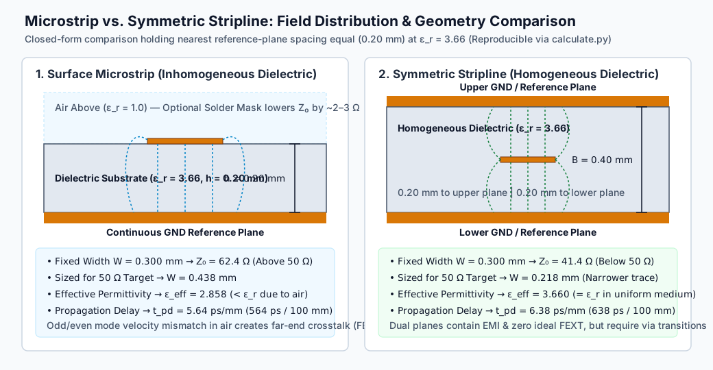
Cross-sectional comparison of surface microstrip and symmetric stripline showing electric field lines, trace widths, and calculated impedance

1. Electromagnetic Physics: How Field Containment Changes Signal Behavior

Before running a stackup field solver, compare how the physical cross-section of each transmission line shapes its electromagnetic propagation (see Texas Instruments KeyStone Hardware Design Guide SPRABI2D, Appendix B and Renesas/IDT Application Note AN-1014):

Engineering Dimension	Surface Microstrip (Outer Layer)	Symmetric / Offset Stripline (Inner Layer)	Practical Design Impact
Dielectric Environment	Inhomogeneous: Substrate ( $ε r$ ) below, air ( $ε r = 1.0$ ) and LPI solder mask ( $ε r \approx 3.3--3.8$ ) above	Homogeneous (or Core + Prepreg): Completely surrounded by dielectric between two reference planes	Microstrip has a lower effective permittivity ( $ε eff < ε r$ ); stripline sees $ε eff \approx ε r$
Propagation Delay ( $t pd$ )	Faster ( $\approx 5.4--6.0 ps/mm$ on typical FR-4 / hydrocarbon laminates)	Slower ( $\approx 6.3--7.2 ps/mm$ on the same dielectric material)	Never match length-for-length in mm when a bus splits across microstrip and stripline layers; match flight time in picoseconds
Far-End Crosstalk (FEXT)	High FEXT: Odd-mode fields travel more in air than even-mode fields ( $v odd \neq v even$ ), accumulating forward crosstalk	Near-Zero Ideal FEXT: Capacitive and inductive coupling match in a uniform medium ( $v odd \approx v even$ )	Stripline allows tighter trace-to-trace pair spacing for the same crosstalk budget (Renesas AN-1014)
Trace Width for $50 Ω$ (at equal nearest-plane spacing $h$ )	Wider trace required (single reference plane provides lower capacitance per unit width)	Narrower trace required (dual reference planes double capacitive coupling, requiring a narrower conductor)	Stripline increases routing density per layer, but narrower copper increases DC and skin-effect conductor resistance
Solder Mask Sensitivity	High: Coating over trace lowers $Z 0$ by $\approx 2--3 Ω$ and adds high- $\tanδ$ mask dielectric loss	Zero: Buried inside internal layers, immune to surface solder mask thickness variation and external handling	Uncoated (solder-mask-relieved) microstrip is often used on $>10 GHz$ RF launches to avoid solder-mask loss
Via Transitions & Stubs	None for surface-to-surface links: Direct connection between top-side SMD pins without vias	Requires $\geq 2$ vias: Signal must drop from L1 pad through vias to inner layer and back up to receiver	Through-hole vias on stripline create resonant open stubs unless routed near the bottom layer or backdrilled

2. Reproducible Geometry Comparison: Same Width vs. Same $50 Ω$ Target

A frequent layout error occurs when an engineer moves a routed $50 Ω$ trace from Layer 1 (microstrip) to Layer 3 (stripline) during congestion cleanup while leaving the CAD trace width unchanged. To illustrate the exact geometric shift without relying on a black-box proprietary solver, we can compare both cross-sections using standard analytical transmission-line equations:

Microstrip Model: Quasi-static Hammerstad–Jensen equations (Qucs Technical Documentation, Eqs. 11.4, 11.6, 11.15–18).
Centered Symmetric Stripline Model: Exact Cohn complete elliptic integral formulation ( $K(k)/K(k')$ ), as implemented in KiCad's coupled_stripline.cpp source and documented in the Polar Instruments Si6000b Technical Appendix.
Controlled Comparison Inputs: Both structures share the exact same distance to the nearest reference plane ( $h = 0.20 mm$ for microstrip; total plane-to-plane spacing $B = 2h = 0.40 mm$ for centered stripline) and a uniform dielectric constant of $ε r = 3.66$ (representative of a hydrocarbon RF laminate's design Dk; see our PCB material datasheet reading guide), under ideal zero-thickness ( $t = 0$ ), uncoated, lossless assumptions.

(Download and run python calculate.py using standard Python 3: calculate.py, calculated-results.csv, and formula notes.)

Experiment 1: Hold Trace Width Constant at $W = 0.300 mm$

When the exact same $0.300 mm$ trace width is placed $0.20 mm$ above one plane (microstrip) versus $0.20 mm$ between two planes (stripline), adding the upper ground plane increases capacitance per unit length and drops characteristic impedance by $21.0 Ω$ :

Topology ( $h nearest = 0.20 mm, ε r = 3.66$ )	Trace Width ( $W$ )	Calculated $Z 0$	Effective Permittivity ( $ε eff$ )	Engineering Takeaway
Surface Microstrip ( $h = 0.20 mm$ , air above)	$0.300 mm$	62.4 Ω	$2.768$	$12.4 Ω$ above a $50 Ω$ target; requires a wider conductor
Centered Stripline ( $B = 0.40 mm$ , dual planes)	$0.300 mm$	41.4 Ω	$3.660$	$8.6 Ω$ below a $50 Ω$ target; requires a narrower conductor

Experiment 2: Synthesize Trace Width for a $50.0 Ω$ Target

Solving both equations for $Z 0 = 50.0 Ω$ reveals the trade-off in conductor width and propagation delay ( $t pd = \sqrtε eff /c$ ):

Topology (Sized for $Z 0 = 50.0 Ω$ )	Required Trace Width ( $W 50Ω$ )	Effective Permittivity ( $ε eff$ )	Propagation Delay ( $t pd$ )	Delay Over a $100 mm$ Trace
Surface Microstrip ( $h = 0.20 mm$ )	0.438 mm	2.858	5.64 ps/mm	564 ps
Centered Stripline ( $B = 0.40 mm$ )	0.218 mm	3.660	6.38 ps/mm	638 ps ( $+74 ps$ slower)

Three practical layout conclusions jump directly out of these numbers:

Width & Copper Loss Tradeoff: At the same $0.20 mm$ distance to the reference plane, the $50 Ω$ stripline trace ( $0.218 mm$ ) is roughly half the width of the $50 Ω$ microstrip trace ( $0.438 mm$ ). While this lets you pack twice as many signals into an internal routing channel, the narrower stripline conductor has higher high-frequency skin-effect attenuation per unit length unless you increase the total dielectric thickness $B$ .
Flight-Time Skew Across Layers: Over a $100 mm$ route, the buried stripline signal arrives $74 ps$ later than the surface microstrip signal ( $638 ps$ vs. $564 ps$ ). On parallel DDR buses or length-matched clock trees that jump between outer and inner layers, always tune delay in picoseconds ( $t pd$ ) rather than physical millimetres.
Why Production Stackups Require a 2D Field Solver: The closed-form $t=0$ model isolates the fundamental topology shift, but a real manufactured PCB adds finite trapezoidal copper thickness ( $t = 18--70 μm$ ), LPI solder mask over microstrip, copper surface roughness ( $R z$ ), and slightly different Dk values between laminated prepreg and core layers in offset/dual-stripline stacks. Never feed the microstrip output $ε eff = 2.858$ back into a 2D field solver's bulk substrate Dk input—supply the laminate's substrate Dk and let the solver compute geometry effects.

3. Evaluating the Whole Channel: Via Stubs, Return Paths, and Insertion Loss

A uniform transmission line segment is only half of the routing decision. Before moving a critical net from microstrip to stripline (or vice versa), evaluate the complete point-to-point channel:

Short Surface RF & Microwave Launches (Favor Microstrip or Grounded Coplanar Waveguide): When connecting an RF transceiver IC directly to a top-side filter, power amplifier, and coaxial/antenna launch over $10--40 mm$ , staying on Layer 1 eliminates two inductive via transitions and via stubs completely. Pulling solder mask back from the RF trace (solder-mask relief / windowing) eliminates solder-mask dielectric loss.
Dense Multi-Gigabit SerDes & Low-Jitter Clocks (Favor Stripline With Stub Control): On long differential channels (PCIe Gen 4/5/6, 25G/56G/112G Ethernet, DDR5) routed across congested boards, outer layers are blocked by component pads and suffer from FEXT and EMI radiation. Routing in internal stripline cavities between continuous GND planes isolates the signals—provided you place return-path ground stitching vias right next to every signal via transition and eliminate long PTH via stubs by routing on deep stripline layers (minimizing stub length) or specifying controlled-depth backdrilling.
Asymmetric / Offset Stripline & Dual Stripline: In high-layer-count boards, placing two signal layers between two reference planes (dual/offset stripline) saves plane layers, but couples the trace more strongly to the nearer plane ( $h 1 < h 2$ ). Route adjacent offset stripline layers orthogonally (or maintain $\geq 3W$ broadside separation) to prevent broadside interlayer crosstalk.

4. Engineering Selection Matrix: When to Choose Microstrip vs. Stripline

Design Constraint or Channel Requirement	Recommended Structure	Key Stackup & Layout Controls to Verify	When to Reject or Modify This Choice
Short RF front-end path requiring probe/tuning access and zero via discontinuities	Uncoated Surface Microstrip (or Grounded Coplanar Waveguide)	Continuous L2 ground plane underneath; specify solder-mask keepout over RF trace; use ENIG/Immersion Ag finish	Reject if dense top-side component placement forces multiple layer jumps or close parallel aggressor routing
High-density SerDes, clock, or parallel bus requiring low FEXT and EMI containment	Symmetric or Offset Stripline	Continuous upper and lower reference planes; place GND stitching vias within $<1--2 mm$ of every signal via transition	Reject or add backdrilling / blind microvias if residual PTH via stub length exceeds $~ λ / (4--10)$ at the Nyquist/harmonic bandwidth
Cost-constrained 4-layer board (`Sig-GND-PWR-Sig`)	Coated Outer Microstrip on L1 and L4	Keep L1 referenced to L2 `GND`; if L4 references L3 `PWR`, place high-frequency decoupling capacitors at via transitions	Avoid routing high-speed differential pairs across splits in the L3 power plane without continuous return reference
Long backplane or server motherboard link with tight insertion-loss budget ( $S 21$ )	Wide-Conducted Stripline in low-loss laminate (e.g., Megtron 6 / Isola / Rogers)	Use thicker dielectric spacing $B$ so $50 Ω / 100 Ω$ traces stay wide enough ( $0.18--0.25 mm$ ) to minimize copper skin loss; specify HVLP/VLP foil	Do not assume stripline has lower total loss than microstrip if thin prepreg forces ultra-narrow ( $0.09 mm$ ) high-resistance inner traces

5. Handing Off Your Stackup and Controlled-Impedance Table for Fabrication

Once your topology and layer assignments are selected, lock the fabrication specification using our controlled-impedance PCB design review checklist. When submitting your PCB manufacturing RFQ, include:

Proposed Layer Stackup & Material Grade: Specifying core/prepreg thicknesses, copper weights (including plated outer copper vs. inner foil), and target laminate family (standard high- $T g$ FR-4, mid-loss, low-loss, or hybrid RF).
Complete Impedance Summary Table: Listing every controlled layer, topology (Coated Microstrip, Uncoated Microstrip, Symmetric Stripline, Offset Stripline, Coplanar), single-ended or differential target ( $Ω \pm %$ ), reference plane layer numbers, and CAD trace width/spacing.
Allowed CAM Trace-Width Adjustment Window: State whether the fabricator's CAM team may adjust controlled-impedance trace widths by $\pm 10--15%$ to match exact pressed prepreg thicknesses and etch factors, or must submit a stackup EQ before altering copper widths.

HILPCB's signal-integrity and CAM engineering team models every multilayer PCB, high-speed PCB, and Rogers RF PCB stackup using 2D field solvers correlated to production press-out data—delivering ±5% TDR impedance control, controlled-depth backdrilling (residual stubs $<10 mil$ ), and sample VNA testing up to 40 GHz. Upload your Gerber/ODB++ files and stackup table when you request a quote for an engineering impedance review.

Frequently Asked Questions

Why is a 50 Ω stripline trace narrower than a 50 Ω microstrip trace at the same dielectric distance?

Characteristic impedance is inversely proportional to capacitance per unit length ( $Z 0 = \sqrtL/C$ ). Because a stripline conductor is coupled to two reference planes (above and below) inside a higher-permittivity dielectric rather than one plane with air above, it has significantly higher capacitance for a given width. To bring capacitance back down and restore $Z 0 = 50 Ω$ , the stripline conductor must be made narrower (or the dielectric spacing between planes must be increased).

Why does microstrip have higher far-end crosstalk (FEXT) than symmetric stripline?

In a homogeneous stripline medium, the electric (capacitive) and magnetic (inductive) coupling ratios between two adjacent traces are equal, so odd-mode and even-mode signals travel at the exact same phase velocity ( $v odd = v even$ ) and far-end crosstalk cancels out theoretically. In surface microstrip, electric field lines fringe into the air above the board; odd-mode fields have a higher fraction of energy in air than even-mode fields, causing velocity mismatch ( $v odd > v even$ ) that produces a large FEXT pulse at the receiver.

How much does solder mask change the impedance of an outer-layer microstrip trace?

Applying standard liquid photoimageable (LPI) solder mask ( $15--30 μm$ thick, $ε r \approx 3.3--3.8$ ) over an outer-layer microstrip trace replaces the air interface directly above the conductor with a higher-permittivity dielectric. This typically lowers single-ended characteristic impedance by $2 to 3 Ω$ (and differential impedance by $3 to 5 Ω$ ), which must be included in the 2D field-solver model before sizing the trace width.

When does stripline perform worse than microstrip at high frequencies?

Stripline can degrade a high-frequency channel in two situations: (1) when transitions from top-layer SMD pads into shallow internal stripline layers leave long through-hole via stubs whose quarter-wave resonance notches out the signal spectrum, and (2) when a tight layer-count stackup forces stripline into ultra-thin dielectrics ( $<0.08 mm$ ), requiring narrow traces ( $<0.10 mm$ ) whose skin-effect and copper-roughness conductor loss exceeds the dielectric loss savings.