
S-parameters describe a channel as ratios of waves leaving and entering its ports, versus frequency. S21, or differential-mode Sdd21, is a complex traveling-wave ratio defined under specified port reference planes, reference impedance, terminations, and mode convention, with other incident waves zero. It is not automatically the fraction of signal or energy delivered in a real transmitter-receiver system. The receiver waveform and eye behavior also depend on the source and load, package, return path, and equalization, as well as nonlinear or time-varying effects that the linear S-parameter model does not include. For a PCB channel, examine transmission, reflection, differential-to-common-mode conversion, and coupling into neighboring lines. A slope, ripple, dip, or rise in mode conversion can suggest a cause, but the plot alone does not establish it.
Before comparing plots, record the port map, normalization, and de-embedding method, along with the reference planes, impedance, terminations, and mode convention. A wrong port map can make crosstalk look like transmission; data quality problems can also undermine simulation results. Measurement setup, coupons and de-embedding are covered in our high-frequency PCB testing guide; this article focuses on reading the result.
1. The Terms That Matter on a Digital Channel
| Term | Meaning | What you want | Plotted as |
|---|---|---|---|
| S21 / Sdd21 (transmission) | Complex transmitted-to-incident traveling-wave ratio with other incident waves zero | Compare with the channel's specified transmission or loss budget over its frequency range | 20 log10|S21| in dB; positive insertion loss is −20 log10|S21| |
| S11 / Sdd11 (reflection) | Complex reflected-to-incident traveling-wave ratio | Compare with the specified reflection limit; a smaller magnitude means higher positive return loss | 20 log10|S11| in dB; positive return loss is −20 log10|S11| |
| Scd21 (mode conversion) | Common-mode output from a differential-mode input | Compare with the applicable interface or design limit | 20 log10|Scd21| in dB |
| NEXT / FEXT | Coupling from an aggressor into a victim at the near or far end | Well below the victim's signal; budget set by the interface | dB |
| Phase / group delay of S21 | Phase and its unwrapped frequency derivative; group delay is −dφ/dω | Compare delay and variation over the required band | phase in degrees; group delay in seconds or ps |
For differential pairs, mixed-mode parameters (Sdd, Scc, Sdc, Scd) complement the single-ended data. Sdd21 is the differential output-to-input traveling-wave ratio under the stated port and reference conditions. Confirm which physical ports form each modal pair and the normalization before comparing files. Scd21 and Sdc21 describe conversion between modes; its effect on emissions or noise susceptibility also depends on the rest of the system.
Port numbering first
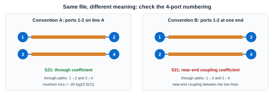
Four-port files are numbered in two common ways: ports 1 and 2 at one end (1→3 and 2→4 are the through paths), or 1 and 2 as the input and output of the first line (1→2 and 3→4 through). S21 describes a through-path coefficient in one convention and a near-end coupling coefficient in the other. Confirm the convention with the person or tool that produced the file before calculating mixed-mode terms.
2. What Insertion Loss Should Look Like
Conductor and dielectric losses generally rise with frequency. Under simplified assumptions, their contributions scale approximately as √f and f, respectively. Actual loss depends on geometry, copper roughness and thickness, and material properties at the frequency of interest. Use a model validated for the stackup and compare representative coupon measurements with the interface budget over its specified frequency range.
| Insertion loss shape | Likely cause |
|---|---|
| Smooth, steeper than expected | Higher Df or rougher copper than modeled, or longer route; check the material and the coupon |
| Ripple superimposed on the slope | Reflections between discontinuities; for two dominant reflections with approximately constant one-way delay, ripple spacing Δf ≈ 1 / (2 × delay) |
| Sharp dip (suck-out) at one frequency | Resonance: via stub at quarter wavelength, or a cavity/plane resonance |
| Dip that moves when the board is touched or the fixture changes | Setup or board sensitivity is possible; use controlled comparisons to isolate the cause |
An ideal open via stub has a first quarter-wave resonance near f ≈ c / (4 L √Dk). With an assumed effective Dk of 3.8, 1.0, 1.5 and 2.5 mm stubs give approximately 38, 26 and 15 GHz. Real geometry and loading shift the result, and the stub can affect transmission below resonance. Backdrilling can shorten the stub and raise its resonance; whether it moves beyond the band depends on the remaining length and structure. See our backdrill guide.
3. Return Loss and Mode Conversion
Positive return loss determines the magnitude of the reflection coefficient: RL = −20 log10|Γ|. The following impedance values are illustrative for a single purely resistive interface referenced to 50 Ω. They are not a unique impedance solution for a general complex load, because the phase of Γ also matters.
| Return loss | |Γ| | Equivalent impedance on 50 Ω |
|---|---|---|
| 10 dB | 0.32 | 26 Ω or 96 Ω |
| 15 dB | 0.18 | 35 Ω or 72 Ω |
| 20 dB | 0.10 | 41 Ω or 61 Ω |
| 26 dB | 0.05 | 45 Ω or 55 Ω |
For the same single-interface model, 47.5 Ω and 52.5 Ω (±5% of 50 Ω) give approximately 31.8 dB and 32.3 dB return loss, respectively. A finite line's result also depends on its length, termination, loss and multiple reflections. Connectors, breakouts, vias and capacitor pads can contribute reflections. A time-domain transform or TDR measurement can help locate discontinuities, subject to bandwidth and resolution; see our TDR testing guide.
As a simplified illustration, consider two matched, uncoupled, lossless paths with a delay difference Δt and consistently normalized differential and common modes. Their differential-to-common transmission magnitude is |sin(π f Δt)| in this ideal model. Real coupling, loss, reflections and port conventions change the result:
| Intra-pair skew | At 8 GHz | At 16 GHz |
|---|---|---|
| 1 ps | −32 dB | −26 dB |
| 5 ps | −18 dB | −12 dB |
| 10 ps | −12 dB | −6 dB |
Skew can arise from unequal routing or material effects. Rising conversion may suggest skew or an asymmetric discontinuity, but it does not identify the cause by itself. Compare the two paths, port mapping and controlled measurements before changing the design.
4. Check the Data Before Using It
| Check | Why | What to look for |
|---|---|---|
| Passivity | A passive network cannot supply net energy | For compatible power-wave normalization, check S-matrix singular values ≤ 1; measurement noise and processing can cause apparent violations |
| Reciprocity | A reciprocal network has a symmetric S-matrix under compatible normalization | Compare Sij and Sji as complex values; investigate differences in the measurement, setup and device |
| Causality | A physical response cannot precede its excitation | Assess with a suitable causality method; finite bandwidth, extrapolation and windowing can produce apparent pre-response |
| Low-frequency start | Time-domain processing may require a DC point or extrapolation | Choose the start frequency and DC treatment for the device and analysis |
| Frequency step | For uniformly spaced data, the step sets the periodic time window: window = 1 / Δf | 10 MHz gives a 100 ns window; check that the window covers the response of interest |
| Upper frequency | Missing high-frequency content can distort a time-domain result | Choose bandwidth for the signal rise time, simulation accuracy and applicable standard; check convergence |
| Reference impedance and format | Touchstone files can use different reference impedances and dB/angle, magnitude/angle or real/imaginary data | Read the option line (# GHz S DB R 50) and any version-specific reference declarations, such as Touchstone 2.0 [Reference], before importing |
| De-embedding | The intended reference planes determine which structures belong in the result | Define the planes and fixture model; validate the selected method and retain any structures required by the test specification |
Many simulation tools report data-quality checks on import. Interpret their results with the method, frequency range and measurement uncertainty in mind.
5. VNA or TDR?
TDR measurements and frequency-domain S-parameters can provide complementary views of a linear channel. A time-domain transform of VNA data can help locate reflections, subject to bandwidth, extrapolation and processing; a TDR trace is likewise limited by the instrument and setup. Available calibration, dynamic range and usable bandwidth depend on the instruments being compared. For the waveform at a receiver, see our eye diagram guide.
6. Specifying S-Parameter Measurements
- Define the structure: coupon or product net, length, layer and reference planes, and the port map.
- Set the sweep: start and stop frequencies and step size based on the standard, signal bandwidth, time window and required accuracy.
- Define calibration and de-embedding: method, fixture files, reference plane.
- State the limits: Sdd21 and Sdd11 masks or values at stated frequencies, mode conversion and crosstalk limits.
- Ask for the data: Touchstone files with the reference impedance and port map stated, not only plots.
For a high-speed PCB, include the stackup, impedance and loss targets, coupon design, frequency range, port map and desired measurements in your quote request. Confirm available materials, tolerances, test methods and deliverables for the specific project before production.
Frequently Asked Questions
What is the difference between S11 and S21?
S11 is the complex reflected-to-incident wave ratio at port 1. S21 is the complex output-to-input wave ratio with other incident waves zero, under the stated port and reference conditions. For a through path, their magnitudes can be expressed as positive return loss and insertion loss, respectively. Neither alone predicts the receiver waveform.
What is Sdd21?
Sdd21 is the complex differential-mode transmission ratio of a differential pair, which can be obtained by converting single-ended four-port data or through a mixed-mode measurement. It is defined with other incident waves zero, for the stated port map, normalization, de-embedding, reference planes, reference impedance, terminations and mode convention. It is not automatically the fraction of signal or energy delivered to a receiver: the receiver waveform and eye behavior also depend on source and load, package, return path and equalization, and linear S-parameters do not include nonlinear or time-varying effects. Compare it with the quantities and limits defined by the applicable interface specification.
How much insertion loss is acceptable?
It depends on the interface's channel budget over its specified frequency range and on the transmitter and receiver. Compare the measured or modeled channel with the applicable limits rather than a universal number.
What causes a dip in insertion loss?
A dip may be caused by a via-stub, cavity or plane resonance, or by a measurement setup issue. Use controlled comparisons and the structure's model to investigate. Shortening a stub can raise its resonance, but the remaining geometry determines whether it is outside the band.
How do I check that an S-parameter file is valid?
Confirm the port map, reference impedance, format and intended reference planes. Check passivity, reciprocity where expected, causality, and the frequency range and step for the intended use. Interpret tool warnings in light of measurement uncertainty and processing.