
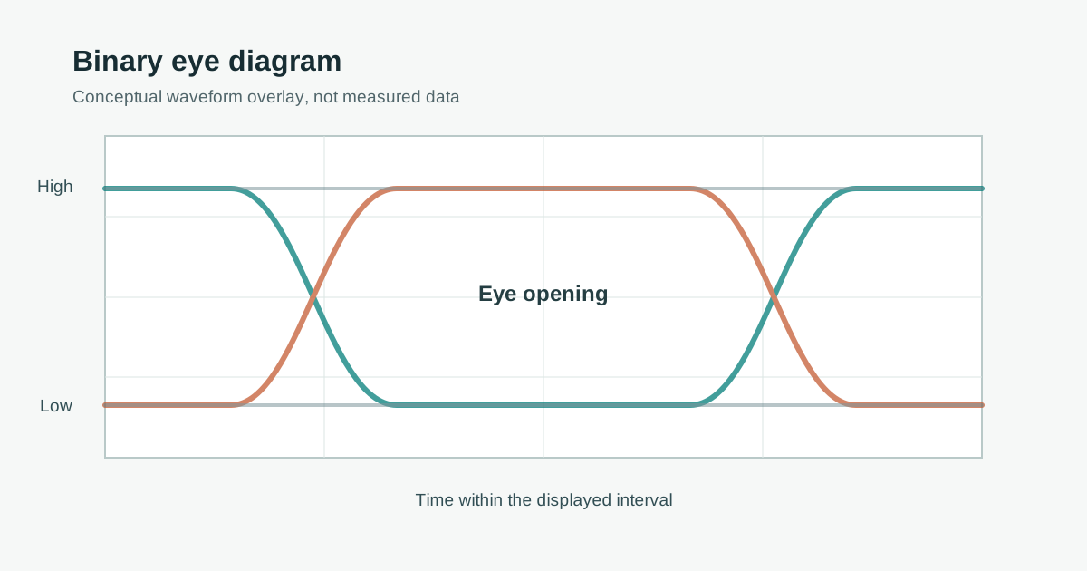
Eye diagrams can be compared only when the measurement plane, pattern, clock recovery, equalization, acquisition and measurement definitions are known. A smaller opening can indicate a channel problem, but it can also result from a different probe or analysis setting; the image alone does not establish the cause or the receiver's error rate.
Compare captures and select the next diagnostic measurement before changing hardware. For channel-wide budgets and release decisions, see waveform integrity in high-frequency PCB channels. When a specification requires a BER contour or mask, record its method and target; a finite raw eye is not automatically an eye at a particular BER.
1. Know the Unit Interval First
The unit interval (UI) is one symbol interval. For binary NRZ, one symbol carries one bit, so the UI equals one bit period; for PAM4, each symbol represents two raw bits before coding overhead. PAM4 has three eyes, and the interface specification defines which eyes and measurement method apply. The examples below use binary signaling.
| Interface | Data rate | UI | Nyquist frequency |
|---|---|---|---|
| DDR4-3200 | 3.2 GT/s | 312.5 ps | 1.6 GHz |
| 10GBASE-R | 10.3125 Gb/s | 97.0 ps | 5.2 GHz |
| PCIe Gen4 | 16 GT/s | 62.5 ps | 8 GHz |
| 25G NRZ | 25.78 Gb/s | 38.8 ps | 12.9 GHz |
| PCIe Gen5 | 32 GT/s | 31.25 ps | 16 GHz |
A 10 ps timing contribution is approximately 3.2% of a 312.5 ps UI and 32% of a 31.25 ps UI. These ratios illustrate the available time scale; they do not establish eye closure or identify a board defect.
2. The Measurements That Matter
| Measurement | Definition | What closes it | Note |
|---|---|---|---|
| Eye height | Vertical opening at a defined sampling window and measurement method | ISI, reflections, crosstalk, power noise | Record the window, population and any statistical contour |
| Eye amplitude | Difference between the measured mean high and low levels | Transmitter swing, channel response and termination | Record the measurement window; amplitude alone does not establish margin |
| Eye width | Horizontal opening at the specified voltage threshold and measurement method | Jitter, ISI, skew within a differential pair | Record the threshold and any BER contour or mask method |
| Crossing percentage | 100 × (crossing − 0 level) / (1 level − 0 level) | Duty-cycle distortion, unequal rise and fall | 50% ideal; 55% means crossings sit high |
| Rise and fall time | 20–80% or 10–90%, per the specification | Loss and dispersion, scope bandwidth | Compare with the same thresholds the spec uses |
| Mask margin | Margin according to the specified mask and scaling method | All of the above | Follow the applicable mask alignment and hit or statistical criteria |
For differential signals, use the differential waveform required by the test. Single-ended measurements of both legs can provide additional evidence of imbalance and common-mode behavior; interpret them with the probe reference and instrument configuration documented.
3. Raw Eye vs BER Eye
One illustrative statistical model represents random jitter (RJ) with Gaussian tails and deterministic jitter (DJ) using a dual-Dirac approximation. Under a specified model and tail convention, an extrapolated total jitter can be written:
Assume a hypothetical 10 Gb/s binary link (100 ps UI), 20 ps DJ and 1.5 ps rms RJ. Using two illustrative tail multipliers, 4.75 and 7.03, define a width as 1 UI minus modeled total jitter:
| Assumed Q | Modeled TJ | Illustrative eye width |
|---|---|---|
| 4.75 | 34.3 ps | 65.8 ps, 0.66 UI |
| 7.03 | 41.1 ps | 58.9 ps, 0.59 UI |
The modeled widths differ by about 6.8 ps. They are not measurements of a real receiver and do not establish compliance. The mapping of Q to a BER depends on the tool's tail and error conventions. The result also depends on decomposition, clock recovery and distribution tails; correlated effects or non-Gaussian tails can invalidate the approximation. A raw acquisition does not become a measurement at 10⁻⁶ merely because it contains millions of bits. For actual acceptance use the interface's specified measurement or extrapolation method, and report error count, bits tested and confidence when reporting measured BER.
4. Rule Out the Measurement First
Measurement setup can alter an apparent eye. Check these conditions before changing the layout:
| Check | Why | Example |
|---|---|---|
| Scope and probe bandwidth | Rise-time estimates depend on instrument response and edge definition | Under a Gaussian-response approximation with system rise time 0.4 / bandwidth, a 20 ps edge estimates 32 ps at 16 GHz and 23 ps at 33 GHz; verify the actual system response |
| Probe loading and ground lead | Probe loading or a long ground lead can introduce or alter ringing | Compare suitable probe arrangements and loading |
| Fixture and cable loss | Adapters, cables and test boards add loss and reflections | Compare at a documented reference plane using validated fixture S-parameters and de-embedding |
| Where you probe | Probing at the receiver pin vs at a via or test point several mm away gives different eyes | Reflections appear or disappear with probe position |
| Reference equalization | Compliance eyes often apply a defined CTLE/DFE; raw eyes do not | A closed raw eye at 16 GT/s may be compliant after reference equalization |
| Pattern length and record length | Short patterns can miss pattern-dependent ISI; short records can miss rare events | PRBS7 vs PRBS31 can give different eye heights on a lossy channel |
| Clock recovery settings | The recovery loop bandwidth defines which jitter is tracked and which is counted | Use the loop bandwidth the specification defines |
5. Eye Symptoms and the Next Check
| Eye symptom | Possible causes | Evidence before a change |
|---|---|---|
| Rounded edges, eye height shrinks with trace length, long-run bits ride higher than single bits | Insertion loss and ISI, or limited measurement bandwidth | Compare channel loss and the measurement response before changing routing, material or equalization |
| Ledges or steps after transitions at a fixed time offset | Reflections, pattern-dependent ISI or fixture artifacts | Check probe position and pattern, then correlate with impedance control and TDR testing |
| Notch or resonance-like closure at specific data rates | Via stubs, connector or fixture resonances | Compare channel and fixture measurements before considering backdrilling or other geometry changes |
| Thick 1 and 0 rails, noise uncorrelated to the data pattern | Crosstalk, power-supply noise or instrument noise | Correlate rails and aggressor activity; see the crosstalk guide |
| Wide crossing region, eye width shrinks, height mostly fine | Clock jitter, ISI or recovery settings | Compare jitter and recovery settings, then correlate clock and supply measurements |
| Crossing not at 50%, or asymmetric edges | Duty-cycle distortion, unequal edges, skew or mode conversion | Compare rising and falling edges and differential and individual-leg measurements |
| Overshoot and ringing at edges | Termination, discontinuities or probe artifacts | Check probing, source/load configuration and TDR before revising termination |
| Double bands on the edges, overshoot above the 1 level | Equalization, pattern dependence or reflections | Compare approved equalization settings and pattern-correlated waveforms |
When one lane differs from its neighbors, compare routing, via count, connector position, settings and measurement setup before attributing the difference to the board.
6. Hypothetical Review: A Lane With a Delayed Feature
Assume a binary 10.3125 Gb/s lane has a 97 ps UI and a feature approximately 35 ps after a transition. This is an illustrative investigation, not a measured customer case. Suppose the team is testing whether a reflection could contribute to the feature:
- Check the setup: document the measurement plane, pattern, bandwidth, clock recovery, equalization and fixture. Compare another suitable measurement setup to investigate probe artifacts.
- Estimate a distance: if 35 ps is a round-trip delay from the reference plane and the assumed one-way propagation delay is 7 ps/mm, then 35/(2 × 7) = 2.5 mm. Real propagation, the reference plane and the feature's origin must be established; this estimate does not locate a particular via or breakout by itself.
- Seek independent evidence: compare TDR and channel measurements with the model, including fixture and package contributions. Examine pattern correlation and alternate causes such as ISI.
- Evaluate a proposed change: only after correlation, compare the relevant geometry or equalization options and repeat the same measurements. An improved eye still needs the interface's prescribed acceptance evidence.
If the delay is not a simple round trip, the estimate is not applicable. Do not treat a visible ledge alone as proof of a board fault or a successful fix.
7. Compare Two Captures Before Changing Hardware
| Comparison field | Capture A | Capture B | Decision |
|---|---|---|---|
| Plane and fixture | Receiver test pad, fixture included | Connector plane, fixture removed | Not directly comparable; reconcile the reference plane and de-embedding |
| Pattern and activity | PRBS7, aggressors idle | PRBS31, aggressors active | Repeat with matched patterns and aggressor state, then vary one condition |
| Clock and equalization | Recovered clock, equalization off | Different recovery bandwidth, reference equalization on | Match the specified settings before attributing the opening difference to hardware |
| Reported result | Finite captured eye | Statistical contour at a stated BER | Preserve both labels; neither alone establishes measured receiver BER |
The rows are hypothetical examples of mismatched conditions, not measurements. Record actual settings, calibration, sample depth, waveform files and any confidence assumptions with each result.
8. Specifying Eye Diagram Verification
- State the interface and specification: data rate, compliance specification and the measurement point (TX pins, RX pins, connector).
- State the method for eye height, width and any BER contour or mask, and whether reference equalization is applied.
- Define the pattern (PRBS length or compliance pattern) and the clock recovery settings.
- Define the fixture and how it is de-embedded.
- Tie the board-level controls to the result: impedance tolerance and coupons, backdrill depth, loss targets.
HILPCB's high-speed PCB catalog lists back-drilling, controlled impedance and advanced VNA, eye diagram and jitter test options. Send the stackup, impedance and loss targets, test plane and measurement requirements in a quote request; confirm the feasible construction, test scope and deliverables for the specific project. The designer owns the channel requirements, the fabricator confirms the board construction and the product owner defines system qualification. For the overall design flow, see the high-speed PCB design guide.
FAQ
What does an eye diagram show?
It overlays repeated intervals of a serial waveform. Eye height, width and crossing behavior describe the opening under a defined measurement method. Loss, reflections, noise, jitter and setup can produce similar symptoms, so use additional evidence to distinguish causes.
What is a good eye height and eye width?
There is no universal number. Use the interface specification's measurement plane, mask or other limits, acquisition or BER method, and any required equalization. A raw opening and a modeled contour are different results and must be labeled accordingly.
Why does my eye look open on the scope but fail compliance?
A finite capture can miss rare events and is not automatically an eye at a particular BER. Compliance tests may use different filters, patterns, clock recovery or a specified statistical method; reconcile those conditions before comparing results.
What causes a closed eye diagram on a PCB?
Insertion loss over long or lossy routes, reflections from impedance discontinuities and via stubs, crosstalk from adjacent signals, power-supply noise, clock jitter, and intra-pair skew. Probe and fixture problems can also look like a closed eye, so check the measurement first.
Do I need an eye diagram if I have TDR and S-parameters?
TDR and S-parameters characterize channel behavior at defined planes; an eye shows waveform behavior under its own source, measurement and processing conditions. An eye may use a reference receiver rather than the actual receiver, and neither measurement alone proves system BER or compliance.