
Jitter is the deviation of signal edges from their ideal timing. A jitter number is only meaningful with three things attached: which metric (period, cycle-to-cycle, time interval error or phase jitter), over what population or band (number of cycles, BER, or integration band and filter), and with what instrument floor. Most disagreements about "how much jitter a board adds" are two people quoting different metrics.
Possible contributors include supply noise reaching the clock source or PLL, crosstalk, channel loss and reflections, and simultaneous switching. A spectral feature or waveform can suggest a cause, but confirm it with controlled comparisons before changing a layout.
1. Pick the Metric for the Question
| Metric | Definition | Use it for | Typical instrument |
|---|---|---|---|
| Period jitter | Deviation of each clock period from a specified reference period | Timing analysis when the device specification calls for this metric | Real-time oscilloscope; use the specified measurement method and sample count |
| Cycle-to-cycle jitter | Change between adjacent periods | PLL and spread-spectrum behavior, some processor clock specs | Oscilloscope |
| Time interval error (TIE) | Each edge's position minus its ideal position | Serial data and reference clocks; the raw data for decomposition and filtering | Oscilloscope with jitter analysis |
| Phase jitter (rms) | Phase noise integrated over a band or through a filter | Reference clocks for SerDes, PCIe, Ethernet; oscillator comparison | Phase noise analyzer, or filtered scope TIE when the method and frequency response are equivalent |
| Total jitter at a BER | A timing spread at a stated BER, measured or estimated by a defined method | Data eye width and link margin | Jitter analysis or BERT as specified; see our eye diagram guide |
Different interfaces define different test points, metrics, filters and limits. PCIe reference-clock requirements, for example, depend on the applicable revision and clock architecture. A filtered result and a generic 12 kHz–20 MHz integration of the same spectrum cannot be compared against each other's limits. Use the applicable interface specification and document its clocking mode, test point and processing.
2. Why Peak-to-Peak Depends on How Long You Look
In an illustrative model, independent edge errors follow a Gaussian distribution with 1 ps rms. Larger samples tend to include more extreme values. The following symmetric quantile spans approximate a sample's scale; they are not exact expected sample ranges or measured results:
| Independent edges assumed | Approximate quantile span |
|---|---|
| 1,000 | ~6.2 ps |
| 10,000 | ~7.4 ps |
| 1,000,000 | ~9.5 ps |
| Actual random jitter need not follow this model, and correlation, edge selection and confidence affect the result. Record the sample count and method with a peak-to-peak value. A finite capture does not establish a particular BER simply from its length. |
3. Decomposing Jitter, and What Each Component Points To
| Component | Character | Typical board-level source |
|---|---|---|
| Random jitter (RJ) | Often modeled with Gaussian tails; reported as rms under a stated method | Device noise and broadband supply or measurement noise |
| Periodic jitter (PJ) | Bounded, at fixed frequencies | Switching regulator ripple coupling into a PLL supply, fan or motor drive, spread-spectrum clocking |
| Data-dependent jitter (DDJ): ISI | Bounded, depends on bit pattern | Channel loss, reflections from impedance steps and via stubs |
| DDJ: duty-cycle distortion (DCD) | Bounded, alternate edges | Asymmetric rise/fall, threshold offset, intra-pair skew |
| Bounded uncorrelated jitter (BUJ) | Bounded in the selected model and uncorrelated to the measured data | Some crosstalk; correlation depends on the aggressor and analysis |
In one dual-Dirac approximation, extrapolated total jitter is written TJ = DJ + 2Q · RJrms. Here DJ and RJ are fitted model parameters; Q depends on the BER and tail convention. Record the fit, transition selection, clock recovery, bandwidth and method. Correlation or non-Gaussian tails can invalidate the approximation; an extrapolation is not a measured receiver BER.
Periodic effects can appear as discrete spurs in a TIE spectrum. A spur near a regulator's switching frequency is a lead, not proof of its origin: check probe coupling, aliasing, harmonics and common sources with controlled comparisons.
4. From Phase Noise to RMS Jitter
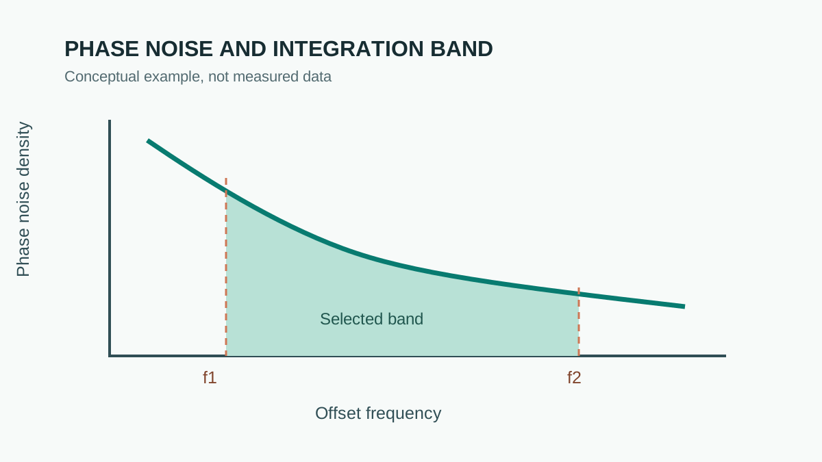
A phase noise analyzer measures single-sideband phase noise L(f) in dBc/Hz versus offset from the carrier. Integrating it over a band gives rms phase jitter:
For a hypothetical 156.25 MHz clock, using the stated single-sideband convention and integrating from 12 kHz to 20 MHz:
| Phase noise profile | RMS jitter |
|---|---|
| Flat −150 dBc/Hz | 204 fs |
| Flat −140 dBc/Hz | 644 fs |
| −125 dBc/Hz to 100 kHz, −135 to 1 MHz, −150 to 20 MHz | 395 fs |
| One −70 dBc single-sideband spur in the band (calculated separately) | 456 fs |
The values illustrate how the spectrum and integration limits affect the result; neither profile nor spur represents a measured board. A discrete spur is specified in dBc rather than dBc/Hz. State whether the instrument includes it in the integral so that it is not counted twice. Applying a compliance filter can produce a different result.
5. Mind the Instrument Floor
When the DUT and independently characterized measurement floor are compatible, uncorrelated rms contributions measured with the same bandwidth, filters and conditions, a corrected estimate can be calculated:
| Measured | Instrument floor | Estimated DUT rms |
|---|---|---|
| 1.2 ps | 0.8 ps | 0.89 ps |
| 0.30 ps | 0.20 ps | 0.22 ps |
| 0.20 ps | 0.15 ps | 0.13 ps |
These are illustrative calculations, not noise-free measurements. Near the floor, uncertainty can dominate. Record the raw result, floor characterization, correction assumptions and uncertainty; correlated noise, deterministic spurs and probe loading cannot generally be removed this way. Select an instrument and probes with adequate sensitivity for the required method, and keep measurement and processing settings consistent across comparisons.
6. Board-Level Causes and Fixes
| Observation | Possible cause | Next check before a change |
|---|---|---|
| Discrete spur at a regulator's switching frequency or harmonic | Supply ripple coupling into the oscillator or PLL, probe coupling or a common source | Compare supply and clock measurements while varying one operating condition; check aliasing and probing. Evaluate filtering and return paths with stability and load requirements; see the power integrity checklist |
| Jitter rises when an adjacent bus or lane is active | Crosstalk, shared supply noise or a measurement interaction | Compare matched captures with aggressors idle and active; see the crosstalk guide |
| DDJ grows with route length and pattern; eye shows ISI | Channel loss, reflections or measurement bandwidth | Compare channel response, pattern and reference plane before considering geometry or equalization changes |
| Jitter correlates with many outputs switching | Supply or ground disturbance, or coupling in the measurement | Compare supply and reference measurements under controlled switching activity |
| Ringing on a clock edge near threshold, period jitter high | Termination, discontinuities or probe artifacts | Check probing and source/load configuration before selecting a termination |
| Clock jitter differs at source and distant load | Clock distribution, loading or different measurement conditions | Match probe and analysis settings, then examine fan-out and routing; see the clock tree layout tutorial |
For an illustrative linear sensitivity of 0.5 ps/mV, 10 mV peak-to-peak ripple corresponds to 5 ps peak-to-peak jitter, provided that sensitivity applies at the ripple frequency and operating point. As a time-scale comparison, 5 ps is 5% of a 10 Gb/s binary UI and 16% of a 32 GT/s UI. Neither ratio establishes compliance.
7. Specifying Jitter Measurements
- Name the metric: period, cycle-to-cycle, TIE, phase jitter or total jitter at a BER.
- State the population or band: number of cycles, BER, integration band or specification filter.
- State the instrument and floor, and whether the floor is removed.
- Define the measurement point and probing method, with the same setup for comparisons.
- Record the operating state: supply source, load and traffic on neighboring interfaces.
HILPCB's high-speed PCB catalog lists controlled impedance, back-drilling and test options. Send the stackup, critical clock and SerDes nets, test plane and measurement requirements in a quote request; confirm the achievable construction, test scope and deliverables for the specific project. For decoupling design around clock sources, see decoupling network basics.
Frequently Asked Questions
What is the difference between period jitter, cycle-to-cycle jitter and TIE?
Period jitter compares each clock period with a specified reference period, often the mean. Cycle-to-cycle jitter is the change between adjacent periods. Time interval error measures each edge against a defined ideal timing reference; the reference and processing determine which variations are included.
How do you convert phase noise to jitter?
Under the stated phase-noise convention, integrate the linear single-sideband noise density over the chosen band, take the square root of twice the integral, and divide by 2π times the carrier frequency. An illustrative flat −150 dBc/Hz from 12 kHz to 20 MHz on a 156.25 MHz clock gives about 204 fs rms. Document filtering and whether spurs are included.
Why does my peak-to-peak jitter increase with longer captures?
In an independent Gaussian model, larger captures tend to contain more extreme edges. Correlation, distribution and edge selection affect the result, so report sample count and method along with the peak-to-peak value. A finite capture does not by itself establish a BER.
What causes jitter on a PCB?
Possible contributors include supply noise at a clock source or PLL, crosstalk, channel loss and reflections, simultaneous switching, and termination. A spur can suggest a source, but controlled comparisons are needed to identify it.
Can an oscilloscope measure femtosecond jitter?
An oscilloscope can be suitable if its characterized floor, bandwidth, probing and uncertainty meet the required method. RSS subtraction is an estimate that requires compatible, uncorrelated contributions; near the floor the uncertainty can dominate. Compare instruments against the actual test requirements.