
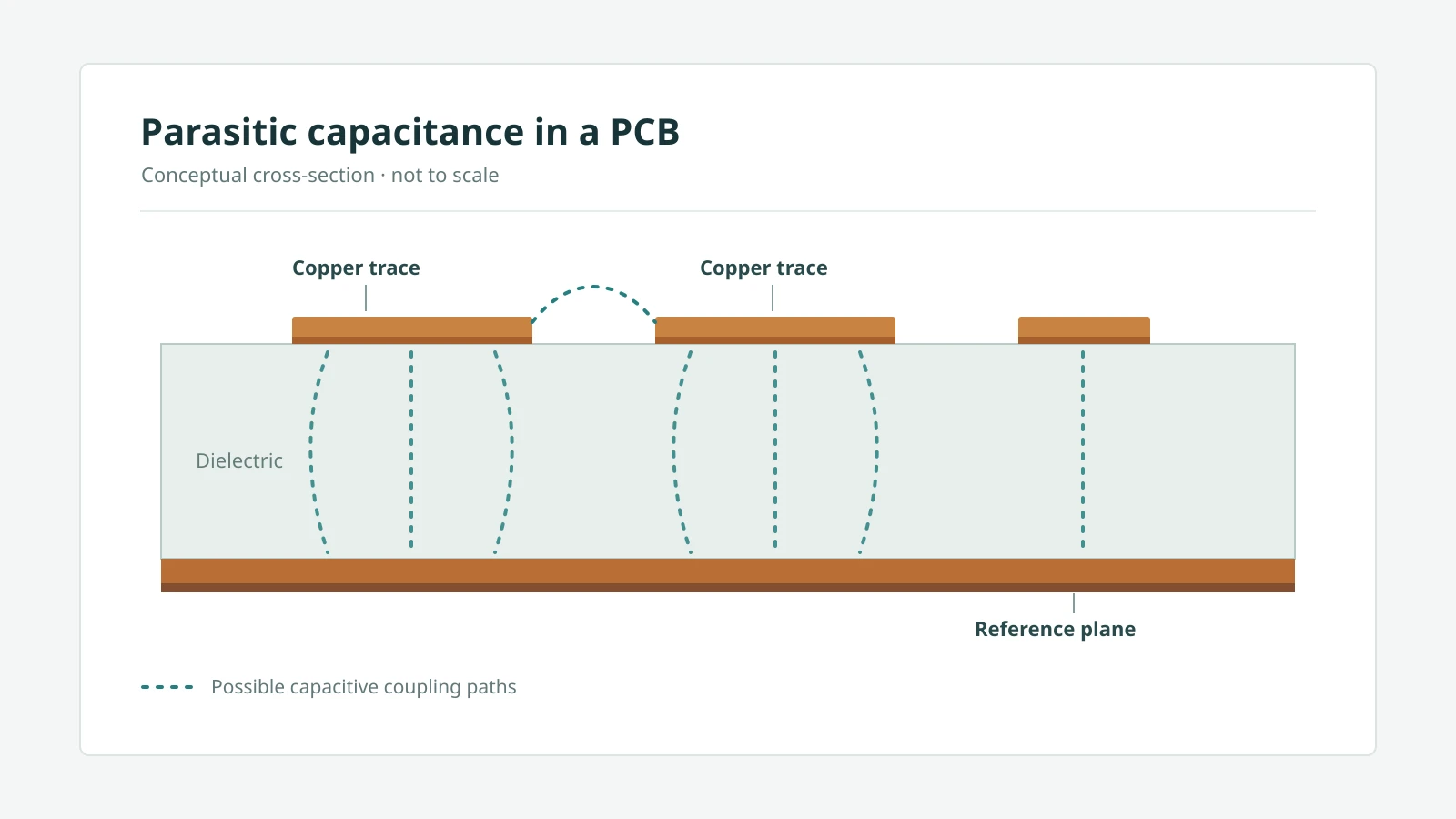
A 0.9 mm by 0.9 mm pad 0.1 mm above a plane has an ideal parallel-plate capacitance of about 0.3 pF. Under one assumed line model, a 50 Ω trace carries about 1.2 pF per centimeter. Actual values depend on geometry, dielectric properties and nearby conductors. Their impact depends on the impedance of the node they load and the signal's edge rate.
In a simple lumped RC model, 0.5 pF with 50 Ω gives a pole near 6.4 GHz; with 1 MΩ it gives a pole near 318 kHz. On a fast channel, a localized capacitance can also create an impedance discontinuity. These are starting points for a capacitance budget, not substitutes for a complete circuit or channel model.
1. Typical Magnitudes: Pads, Vias and Traces
Conductors couple to nearby conductors, including planes and adjacent traces. The estimates below use the stated geometries and dielectric assumptions; other coupling paths may also matter.
Pad to plane
A pad over a plane behaves approximately as a parallel-plate capacitor:
C = (epsilon_0 * epsilon_r * A) / d
The table assumes an ideal, continuous plane, epsilon_r = 4.2, and the listed pad areas and separations. It does not predict a particular package or a plane cutout.
| Assumed pad | Area | 0.1 mm to plane | 0.2 mm to plane | 1.3 mm to plane |
|---|---|---|---|---|
| 0402 land, 0.5 × 0.6 mm | 0.30 mm² | 0.11 pF | 0.06 pF | 0.01 pF |
| 0603 land, 0.9 × 0.9 mm | 0.81 mm² | 0.30 pF | 0.15 pF | 0.02 pF |
| Edge-launch connector pad, 1.5 × 3.0 mm | 4.5 mm² | 1.67 pF | 0.84 pF | 0.13 pF |
The parallel-plate model ignores fringing and other conductors. Use it for an initial comparison; evaluate the actual stackup and geometry with a field solver or measurement when the result matters. A local plane cutout has different fields from the ideal continuous plane in the last column and also affects the return path.
Via barrel to plane antipads
Via geometry, plane clearances, layer transitions and unused barrel length all affect the response. A simplified estimate can help compare geometries, but it cannot fully represent a distributed via and its return path. See our via capacitance guide for the estimate and its assumptions; TI's high-speed design guidance also discusses via design.
Trace to plane
For a uniform, approximately lossless quasi-TEM line, capacitance per unit length can be estimated from characteristic impedance and effective dielectric constant:
C' = sqrt(epsilon_eff) / (c * Z0)
| Assumed line | epsilon_eff |
Capacitance per cm |
|---|---|---|
| 50 Ω microstrip | 3.3 | 1.21 pF/cm |
| 50 Ω stripline | 4.2 | 1.37 pF/cm |
| 100 Ω trace (single-ended) | 3.3 | 0.61 pF/cm |
These examples use the assumed impedance and effective dielectric constant at the frequency of interest; real lines can be dispersive and lossy. Line capacitance is part of Z0, not automatically a defect. Extra capacitance can matter at a stub or on a sensitive amplifier input.
2. When It Matters: Two Quick Tests
Parasitic capacitance is a problem in two distinct situations, and each has its own test.
Test 1: high-impedance nodes (RC pole)
A simple node with Thevenin resistance R and total capacitance C has a pole at:
f_3dB = 1 / (2 * pi * R * C)
| Node resistance | 0.5 pF | 2 pF | Typical node |
|---|---|---|---|
| 50 Ω | 6.4 GHz | 1.6 GHz | RF port, terminated line |
| 1 kΩ | 318 MHz | 80 MHz | Fast amplifier feedback network |
| 10 kΩ | 32 MHz | 8 MHz | Precision amplifier gain resistors |
| 100 kΩ | 3.2 MHz | 0.8 MHz | Low-power regulator feedback divider |
| 1 MΩ | 318 kHz | 80 kHz | Sensor, photodiode, electrometer input |
| 10 MΩ | 32 kHz | 8 kHz | pH, charge or leakage measurement |
Compare the pole with the required bandwidth and error budget. At an amplifier's inverting input, capacitance also interacts with the feedback network and can reduce phase margin; assess stability using the specific amplifier, circuit and load.
Test 2: fast edges (discontinuity time constant)
For a zero-length shunt capacitance C between matched lines of equal impedance Z0, an ideal incident step has a single-pole response with time constant:
tau = (Z0 * C) / 2
Before a far-end reflection returns, the ideal step response has a 10–90% transition time of approximately 2.2 * tau:
| Lumped C on matched 50 Ω lines | tau |
Ideal step response, 10–90% |
|---|---|---|
| 0.2 pF | 5 ps | ~11 ps |
| 0.5 pF | 12.5 ps | ~28 ps |
| 1.0 pF | 25 ps | ~55 ps |
This is not a time to add directly to an input edge that already has a finite rise time. Compare the scales as a screening step, then use the actual waveform and a suitable channel model or measurement to assess reflections and edge shape.
3. Worked Example: Switch Node Coupling Into a Regulator Feedback Pin
A hypothetical buck regulator switches its SW node between 0 V and 12 V at 2 MHz. Its feedback divider sets 0.8 V at FB. Assume 0.05 pF of coupling from SW to FB and 5 pF from FB to ground; these are illustrative values, not measurements.
For an instantaneous SW step in a linear lumped model, the initial FB disturbance is the capacitive-divider estimate:
Delta V_FB = V_SW * C_c / (C_c + C_node) = 12 V * 0.05 / 5.05 = 119 mV
That initial estimate is about 15% of 0.8 V. With an ideal resistive return, its decay time constant depends on the divider's Thevenin resistance:
| Divider | R_th |
tau = R_th * (C_c + C_node) |
Relative to the 500 ns period |
|---|---|---|---|
| 100 kΩ / 20 kΩ | 16.7 kΩ | 84 ns | About 0.17 periods |
| 1 MΩ / 200 kΩ | 167 kΩ | 842 ns | About 1.68 periods |
The actual response also depends on edge duration, duty cycle, successive edge polarities, feedback dynamics and other parasitics. The time constants alone do not establish settling or instability. Consider these layout measures and verify the result against the regulator datasheet and circuit behavior:
- Route FB away from SW copper, and keep it on the opposite side of a ground plane or with ground copper between them.
- Place the divider next to the FB pin, so the high-impedance trace is millimeters long and the long run to the output is low impedance.
- Add a small feed-forward or filter capacitor only if the regulator datasheet recommends one, because it changes loop compensation.
The coupling value here is a representative layout estimate, not a measurement. Field solvers or the regulator vendor's layout guide give the numbers for a specific geometry.
4. Fast Edges: Where Discontinuity Capacitance Comes From
On high-speed channels the concern is often excess capacitance: capacitance beyond what the transmission line's Z0 already accounts for in a chosen model. Possible sources include:
| Structure | Why it adds excess capacitance | Typical layout response |
|---|---|---|
| Connector or edge-launch pad | Pad much wider than the 50 Ω trace | Evaluate a plane cutout and model the complete launch and return path |
| AC-coupling capacitor and BGA pads | Pad wider than the trace, close to the plane | Plane cutout under pads, sized from simulation |
| Signal via | Barrel and pads load the planes it passes | Larger antipads, remove non-functional pads, ground return vias nearby |
| Via stub | Unused barrel length acts as an open stub and resonates | Backdrill or use blind/buried vias (see our backdrill guide) |
| Test points and stubs on the line | Extra copper hanging off the line | Keep stubs minimal or move test access to a low-speed point |
Fixes often trade capacitance against inductance. A larger antipad can reduce via capacitance while changing return-path coupling and the apparent inductive response. Evaluate the complete transition for the target impedance, rather than minimizing capacitance alone. For impedance targets and how they are measured, see our characteristic impedance guide.
5. Reduction Methods and What Each One Costs
Every reduction technique moves something else. Pick the method from the test that failed in section 2, then check the side effect.
| Method | Capacitance effect | What it costs | Best used for |
|---|---|---|---|
| Plane cutout under a pad | Can reduce coupling to the nearest plane | Changes the return path and fields; neighboring traces should not cross the void | Connector launches, AC-coupling caps, RF pads, sensitive input pads, after modeling |
| Larger via antipads | Can reduce via-to-plane C | Changes return coupling and inductance; leaves less plane copper between vias | High-speed signal vias, tuned with simulation |
| Remove non-functional inner pads | Lowers via C and pad-to-plane loading | Fabricator approval needed; affects drill and plating process | Dense BGA fan-outs, high-speed vias |
| Backdrill or blind/buried via | Can reduce unused stub length and its resonant effects | Added process step and drawing callouts; backdrilling leaves a specified residual stub | Channels where stub simulations or measurements warrant it |
| Thicker dielectric to the plane | Reduces ideal parallel-plate C for fixed area | Changes trace impedance, return paths and coupling | Stackups evaluated as a whole |
| Lower-Dk laminate | Can reduce capacitance; the result depends on geometry and field distribution | Material cost, lead time and changed impedance | RF and high-speed boards already choosing a laminate |
| Shorter high-impedance traces | Lowers trace C directly | Placement constraints | Amplifier inputs, feedback dividers, crystal pins |
| Distance or a grounded guard between aggressor and victim | Can reduce direct coupling | May add C to ground on the victim; guard connections and geometry matter | Coupling from switch nodes or clocks into sensitive nodes |
| Driven guard held near the node's potential | Can reduce effective loading and leakage | Requires a suitable stable driver; effectiveness depends on frequency and layout | Electrometer, pH, photodiode and leakage-sensitive inputs |
Guard traces have their own rules for when they help and when they hurt. See our guard trace design guide. For coupling between parallel traces, see our crosstalk guide.
Moating and plane cutouts: keep the return path
A plane cutout changes the nearby fields and return path. Evaluate the whole transition, including the replacement reference and any adjacent signals:
- Avoid routing other signals across the void. A missing reference can increase discontinuity and radiation.
- Plan the reference transition. Where appropriate, connect reference planes with nearby ground vias and validate the resulting return path.
For return path planning, see our return path design guide.
6. Estimating Excess Capacitance With TDR
TDR records a reflection, not capacitance directly. Extracting capacitance from that response is a model-dependent estimate; it is not necessarily total capacitance or a unique decomposition into physical inductance and capacitance.
In “Measuring Parasitic Capacitance and Inductance Using TDR”, David J. Dascher derives a model for a discrete shunt capacitor between matched lines of equal impedance. For that model, the signed reflected voltage, with the settled incident level removed and normalized to the incident step height at the discontinuity, is integrated. Raw combined-voltage, percent-reflection and impedance displays require the applicable conversion. The result and factor depend on the topology.
Define the baseline and integration window, capture the response through settling, and check sensitivity to the window. If the settled reflection is nonzero, document how it is treated. A short distributed feature may be represented by a single excess element relative to the line only within the chosen model; neighboring mixed features cannot always be separated by a visual dip.
Measurement resolution must be sufficient to separate relevant responses. This is distinct from whether a single lumped-element model is valid, which is best suited when the transition time is long compared with the feature's propagation delay. Finite bandwidth, loss, windowing and overlapping reflections limit the extraction.
Document calibration or correction, the reference plane, fixtures, probes and cables, rise time, losses, reference accuracy and repeatability, as discussed in Tektronix's TDR measurement guidance. Project evidence should also record uncertainty or sensitivity, the actual data, extraction method, model and limitations. See our TDR testing guide and PCB test coupons guide.
7. Fabrication Notes and RFQ Checklist
Most parasitic-capacitance decisions in layout depend on the fabricator building exactly the stackup and copper shown. State these on the drawing:
- Dielectric thickness and dielectric constant per layer, with the tolerances used in your model.
- Intentional plane cutouts and keep-outs. Mark them as deliberate so CAM does not fill them with copper thieving or balancing pours (see our copper thieving guide).
- Non-functional pad handling. State whether CAM may remove or must keep inner non-functional pads.
- Antipad sizes as drawn. Ask to be told before any change for drill or registration reasons.
- Backdrill nets and maximum residual stub, if used.
- Impedance control and evidence. Specify line targets and tolerances, coupon and TDR report requirements for agreement with the fabricator.
For available high-speed PCB and high-frequency PCB options, send your stackup, Gerber or ODB++ data and impedance requirements with a quote request. Agree on cutouts, antipads, non-functional pad handling, backdrill limits and any test reports for the specific order.
FAQ
How much capacitance does a PCB via add?
It depends on the via, stackup, clearances and nearby conductors. A simplified calculation gives an initial estimate; a field solver or a measurement interpreted with an appropriate model can refine it. See the via capacitance guide.
When does parasitic capacitance actually matter?
At a high-impedance node, compare the simple RC pole with the required bandwidth: 0.5 pF and 1 MΩ give about 318 kHz. For a shunt 0.5 pF between matched 50 Ω lines, the ideal step response has a 10–90% time of about 28 ps. That is not a fixed increment to a finite input rise time.
Why cut the ground plane under a pad?
A cutout may reduce coupling to the nearby plane, but it also changes the return path. Avoid routing other signals across the void and model or measure the complete transition, including any reference-plane connections.
Does a lower-Dk material reduce parasitic capacitance?
It can, but the effect depends on geometry and field distribution. Proportional scaling is a simplification for fixed geometry and a uniform dielectric; practical pads, vias and traces may have fields in multiple materials. Recheck impedance and the complete stackup.
Why does TDR give a different capacitance than an LCR meter?
An LCR measurement includes the structure and fixture contributions within its measurement setup and frequency range. TDR records a reflection from which excess capacitance may be estimated relative to a line model. Different reference planes, frequency ranges, fixtures and extraction assumptions can produce different results.